

Last Updated on
Excel is a spreadsheet software program that allows you to create and edit tables, charts, graphs, and formulas. The program also has a built-in database function that lets you store data from other sources.
You can easily compare two columns in Excel using the IF() formula. This formula compares two values and returns either TRUE or FALSE depending on whether they match.
Compare Two Columns For Exact Row Match
This method is the easiest way to compare columns. For this method, you need to do a row-by-row comparison. From these comparisons, you can then discover which rows share the same data compared to those that don’t.
Step
Use Formula
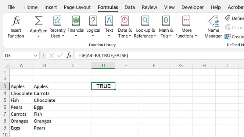
To do so, use the following formula:
IF(A1=B1,”TRUE”,”FALSE”)
If A1 equals B1, then it will return TRUE, otherwise, it will return FALSE.
Compare Two Columns For Partial Matches
The next step up from the previous example is to compare two columns for partial matches. This means that some cells are equal, but others are different.
Step
Use Formula
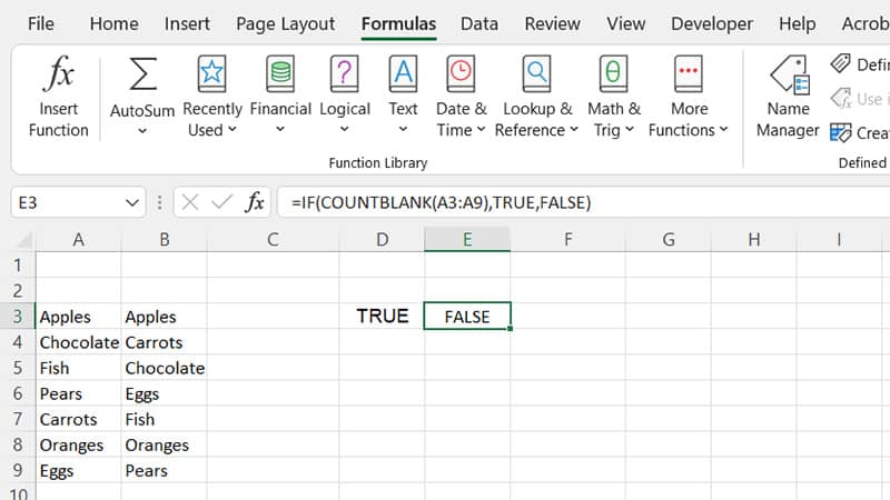
If you want to find out if any of the cells in column A are equal to any of the cells in B, you would use the following formula:
IF(COUNTBLANK(A3:A9), TRUE, FALSE)
This formula counts the number of blank cells in column A (A1 through A10). If there are no blank cells in column A, then it will return FALSE. Otherwise, it will return TRUE.
Compare Two Columns For Similar Values
We then come to compare two columns with similar values. You might be tempted to think that this is just like the previous one, except instead of counting the blanks, you count the non-blank cells.
However, this could lead to problems because sometimes there may be more than one cell with the same value.
For instance, if you had three cells each containing “123”, the COUNTBLANK() formula would only see them as having one cell with 123. Therefore, we must take into account all the cells with the same value.
To do this, we use the SUMPRODUCT() function. This function takes multiple arguments and adds their results together.
Step
Use SUMPRODUCT ()
We use SUMPRODUCT () to add up all the cells in both columns.
Step
Divide The Result
Then we divide this result by the total number of cells in column A. This gives us an average value per cell.
Step
Test
Finally, we test this against 0.
If the average is greater than zero, then we know that at least one cell in column A contains a value that appears in column B. The following formula accomplishes this task:
SUMPRODUCT((A3:A9)*(B3:B9)).
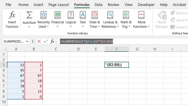
In this formula, the first argument is the range of cells in column A; the second argument is the range of values in column B, and the third argument is the multiplication operator. The multiplication operator multiplies the contents of the two ranges together.
The sum of these numbers is divided by the total number of values in column A. This calculation tells us how many times the value in column A occurs within column B.
Compare Two Columns And Highlight Matches
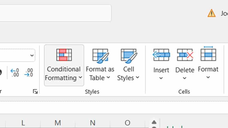
When comparing columns, you can use the ‘duplicate’ function in Conditional Formatting to highlight matching values. This is different from what we’ve seen when comparing rows. In this case, there are no rows being compared, so we’ll need to do something else.
Step
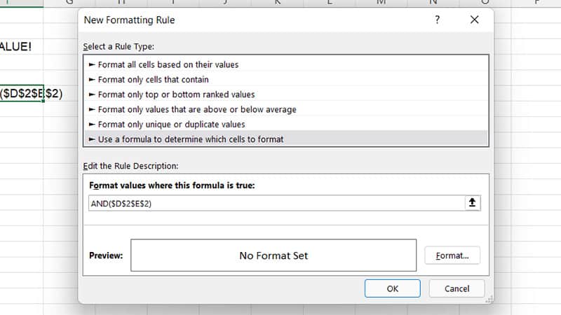
Create A New Rule
Create a new rule based on our original conditional formatting rule. We simply change the condition to check for duplicates rather than blanks. For example, if you wanted to highlight duplicate values, you’d set your conditional format rule to look like this:
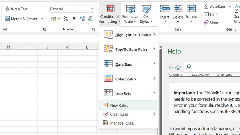
AND($D$2$E$2)
The $D$2 part says that we’re looking for duplicates in column D. The $E$2 part says that the value in column E should match the value in column D.
Step
Apply New Rule
Now, we have to tell Excel which cells to apply the new rule to. A way to do this is by choosing ‘Conditional Formatting’ from the list on the left side of the dialog box. Click ‘New Rule’ and enter the name of the rule in the ‘Name’ field. The rest will be done for you!
Final Thoughts
As long as you have the appropriate formulas, then you can compare columns in Excel in a number of ways. We hope this article has provided you with guidance on how to do this.