

Last Updated on
If you don’t want anyone else to edit your data, then learning how to lock rows in Excel is essential.
However, if you’re new to Excel, you might be wondering: How do you lock a row in Excel?
In this article, I will explore how to lock rows in Excel.
Without further ado, let’s get into it.
When working with spreadsheets and a large amount of data, things can get complicated very quickly.
However, there are ways of comparing data that make the process much smoother and generally less stressful.
Depending on the task at hand, locking a row is a super handy tip to learn. For instance, this is particularly true when comparing two different sets of data that are nowhere near each other on your spreadsheet.
One of the easiest ways to achieve this is to freeze a row (or column). In short, freezing rows means that regardless of where you scroll in the sheet, the particular rows or columns that have been frozen always remain visible in the same place. This means that you’re still able to move the rest of the spreadsheet up or down or side to side.
Why Should You Lock Rows In Excel?
Scrolling for minutes at a time to try to compare two sets of data isn’t an efficient way of working. So, this is why people make use of locking rows in Excel!
After all, you don’t want to spend an unnecessary amount of time searching for data when you could have it right in front of you at all times.
How To Lock A Row In Excel
Learn how to lock rows in Excel.
Step
Scroll Down Excel Sheet
To begin, you will first need to scroll down on the Excel sheet until you find the row that you’d like to lock is the first row that is under the row of letters.
Step
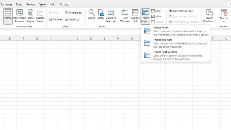
Click On View
Next, you need to click “View” in the menu.
Step
Freeze Top Row
Once you’re in “View” you will need to click the “Freeze Panes” window followed by “Freeze Top Row.”
How To Freeze Multiple Rows In Excel
Learn how to freeze multiple rows in excel.
Step
Select Rows
To start, you will need to select the row below the set of rows that you wish to freeze.
Step
Click On View
In the menu, you will need to click “View.”
Step
Freeze Panes
Once you’re in View, you will need to click the “Freeze Panes” menu and then click “Freeze Panes.”
How To Release A Row In Excel
Once you have frozen a row in Excel, you can easily release a locked row again after you’ve carried out your task.
Step
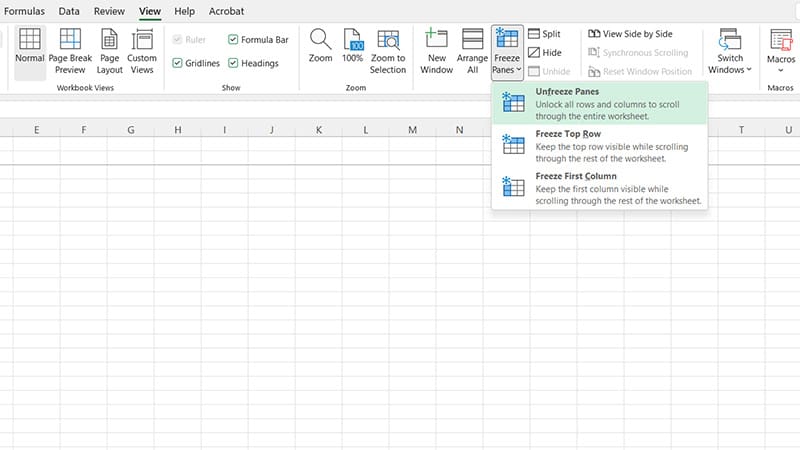
Return To Freeze Panes
Simply return to the “Freeze Panes” menu.
Step
Unfreeze Row
Click “Unfreeze” to release the desired row in Excel.
What Is An Excel Pane?
Many people like to compare Excel panes to window panes in a house! Each section in a window regardless of size can be called a pane.
In short, then, an Excel pane is a set of columns and rows similar to a window. Although it’s more complex than this, this is just a simple way of thinking about it.
Within Excel, you have the option to freeze, unfreeze, or split panes.
Freezing panes in Excel allows you to compare data much more easily, as this just means that the data will remain visible no matter how much you scroll on the spreadsheet.
Conclusion
Locking (freezing) rows in Excel allows you to carry out a variety of tasks much more easily.
If you have selected all the rows that you wish to be locked (or frozen) then you can easily use the Freeze Panes menu to help you achieve this.
Good luck locking a row in Excel!