

Last Updated on
Microsoft Excel has a large array of tools for organizing and managing data. And there may be times when you have a set of data arranged neatly in a column, but need to switch it to be organized in a row. In other words, you may want to Transpose in Excel. Altering the orientation of a set of cells isn’t hard and can be achieved using this function.
This can be a useful skill for quickly rearranging the way your sheet is organized, without copying and pasting the data cell by cell into the new arrangement you want. In this guide, we will tell you how to use the transpose function to rotate a collection of cells.
Rotating Cells In Excel With The Transpose Function
Switching a batch of cells from a column to a row can have a number of useful applications for organizing your spreadsheet.
Step
Highlight Horizontal Row Of Empty Cells
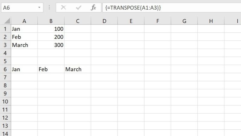
The first thing you will need is a column of numbers with names attached to them.
Highlight a horizontal row of empty cells, making sure to highlight enough to contain all the information in your column.
So, for example, if we had four names and four numbers allocated to each, then you would need to highlight 8 cells in total.
Step
Type =TRANSPOSE
While these cells are highlighted, type ‘=TRANSPOSE(‘ to begin your formula. You will then be able to type the range of cells that contains the column you want to transpose.
So if you had your list of names begin in B2 and end at C5, then you would enter the formula ‘=TRANSPOSE(B2,C5)’.
This formula specifies both the columns of cells containing your list and indicates that these are the cells you want to transpose.
Step
Transpose
When you are done, press ‘CTRL+SHIFT+ENTER’ to confirm your formula and transpose your cells.
How To Transpose Cells Using Copy And Paste
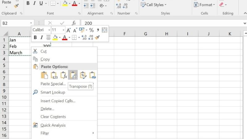
If you want to alter the orientation of a batch of cells, without changing the formatting of the text contained within, then you can do so using copy and paste.
Step
Select The Batch Of Cells
Select the batch of cells that you want to transpose and copy, or cut them. You can do this by right-clicking, or using the key commands ‘CTRL+C’ or ‘CTRL+X’ respectively.
Step
Transpose Option
Now highlight the batch of cells that you want to transpose your data into. Right click once you have highlighted your selection and look for the ‘Transpose’ option in ‘Paste Options’.
You can then click this option and your data will be rearranged. Using this method will create duplicates that you may need to delete afterwards.
You don’t always need to manually type the range of cells that you want to transpose. Instead, after typing ‘=TRANSPOSE(‘ you can highlight the set of cells you want to re-orientate with your cursor. Just remember you have to press ‘CTRL+SHIFT+ENTER’ rather than just ‘ENTER’ on its own.
If you are transposing cells that contain formulas, then the formulas should be automatically adjusted to apply to their new cells.
Final thoughts
The transpose in Excel function isn’t difficult to use and can be made even easier with a few simple tricks. You can use this function to turn a column of cells into a row, or a row of cells into a column, so it works both ways.
The transpose function is one of the simplest array formulas in Excel and is very useful when quickly making changes to the layout of your spreadsheet. Learning about other array formulas will give you lots of other useful tricks that you can use to master your data.