
Last Updated on
Grid lines in Excel are incredibly useful, helping you distinguish between the different cells of a spreadsheet.
However, there may be times when you want to hide or otherwise get rid of the lines of the grid on your worksheet.
This guide will show you how to hide that grid line pattern on virtually any type of Excel worksheet.
What Are Grid lines In Excel?
Grid lines are the thin gray lines that separate cells from each other on a spreadsheet. These help a user differentiate between the various rows and columns in most spreadsheet programs, including Google Sheets and Microsoft Excel.
As we have already mentioned, grid lines are useful for keeping the alignments of rows and columns easily visible.
And there are a few methods that you can use for hiding the grid lines on the worksheet that you are currently using. Let’s go through them.
Using the Hide Option In Your Excel Ribbon
This is an option that you can use in virtually all versions of Microsoft Excel to hide grid lines in Excel – although where it is located varies between versions.
Step
Excel 2007 – Present
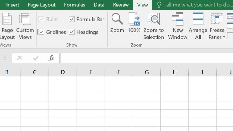
In a modern version of the program, and dating back to 2007, Excel gives you the option to simply hide the grid lines in your ribbons at the top of the program.
All you need to do is simply press the ‘View’ tab, then select the option that says ‘grid lines’ in the ‘Show’ section. This will uncheck the grid lines from your spreadsheet.
Alternatively, you can also change the option in your ‘Page Layout’ tab, in the ‘Sheet Options’ Section.
You can also choose whether the grid lines are visible in the printed version of a worksheet from this section.
Step
Excel Version 2003 And Older
In this version, you need to navigate the program to ‘Tools’, then the ‘Options’ choice.
From here, a drop-down box will appear, giving you a range of options to modify. For our purposes, go to the ‘View’ tab of the new window, navigate to the ‘Window option’s section, and tick/untick the grid lines option.
Change The Color Of The Spreadsheet
It’s also possible for you to simply change the color of the page so that the grid lines match the color of the worksheet itself.
Below are the steps on how to change the color of the spreadsheets
Step
Click The Fill Color Option
For this option, make sure that all the cells of the sheet are selected.
Then click the ‘Fill color’ option at the top of the ‘Home’ tab on the program ribbon.
Step
Select White And The Entire Sheet Will Be A Single Color
Once you have done this, select white and the entire sheet will be a single color, including the grid lines.
Use VBA Script To Hide Spreadsheet Grid Lines
This option relies on modifying the code of Microsoft Excel by using a specific macro.
Below are the steps on using VBA Script to hide spreadsheet grid lines.
Step
Press The View Code Button
For this option, you just need to press the ‘View code’ button on your keyboard whilst you are in Microsoft Excel.
Step
Input Hide_Mech
Then by inputting ‘Hide_Mech’ you can hide the grid lines of a worksheet.
However, keep in mind that if you have already hidden the spreadsheet’s grid lines through some other means, the code window will state ‘Grid Lines are already hidden!’
Final Thoughts
As you can see, while some of the options we have mentioned can be a little complicated, there are plenty of ways for you to remove or add back the grid lines on your Excel worksheet.
- Check out more of our guides on Excel for the best functions and top tips.